Collaborative live-coding with GPU

So, I wanted to combine teaching GPU computing in Python with collaborative notebooks. I got the idea of combining Numba, that I started exploring here, with a notebook that I could use in class with collaborative editing. As I mentioned earlier, I wanted to try out Google Colaboratory with its Jupyter-like notebooks. Google Colaboratory actually offers GPU support in their runtime, so this looked like the perfect match.

Well, so far I have not been able to make it work. It seems that the CUDA toolkit is not installed in the runtime environment from the beginning, so I had to find a way to do that. I have tried two approaches so far:

1. Use pip to install Numba and then install the CUDA toolkit from NVIDIA’s repository using apt.
2. Install Anaconda’s Miniconda installer and then use that to install Numba and the CUDA toolkit.

The good news: both approaches seem to work for installing the library/package. However, so far I cannot get any of it to run…

1. pip and apt

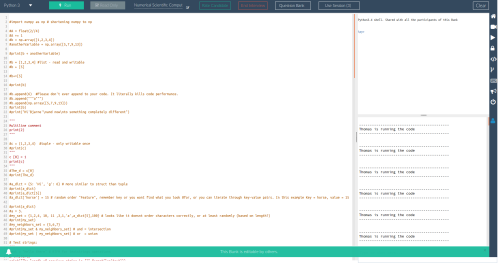
So this is what I have tried so far in a Google Colaboratory notebook.

First, installing Numba is straight-forward:

!pip install numba

Then I install CUDA from NVIDIA’s instructions. This works almost out of the box:

!wget http://developer.download.nvidia.com/compute/cuda/repos/ubuntu1604/x86_64/cuda-repo-ubuntu1604_9.1.85-1_amd64.deb
!dpkg -i cuda-repo-ubuntu1604_9.1.85-1_amd64.deb

Then I had to install the dependency dirmngr as well:

!apt install dirmngr

…and then continuing from NVIDIA’s instructions:

!apt-key adv --fetch-keys http://developer.download.nvidia.com/compute/cuda/repos/ubuntu1604/x86_64/7fa2af80.pub
!apt-get update
!apt-get install cuda

All of this went fine so far, but then I tried to run a Numba example:

import numpy as np
from numba import vectorize

@vectorize(['float32(float32, float32)'], target='cuda')
def Add(a, b):
    return a + b

# Initialize arrays
N = 100000
A = np.ones(N, dtype=np.float32)
B = np.ones(A.shape, dtype=A.dtype)
C = np.empty_like(A, dtype=A.dtype)

# Add arrays on GPU
C = Add(A, B)

Unfortunately Numba throws an error and complains:

---------------------------------------------------------------------------
OSError                                   Traceback (most recent call last)
/usr/local/lib/python3.6/dist-packages/numba/cuda/cudadrv/nvvm.py in __new__(cls)
    110                 try:
--> 111                     inst.driver = open_cudalib('nvvm', ccc=True)
    112                 except OSError as e:

/usr/local/lib/python3.6/dist-packages/numba/cuda/cudadrv/libs.py in open_cudalib(lib, ccc)
     47     if path is None:
---> 48         raise OSError('library %s not found' % lib)
     49     if ccc:

OSError: library nvvm not found

It seems nvvm was supposed to be part of the CUDA toolkit, but it is nowhere to be found…

2. Anaconda

Then I decided to try using Anaconda instead since I know the CUDA toolkit is available here and straight-forward to install using the conda package manager. I started by downloading and installing Miniconda:

!wget https://repo.continuum.io/miniconda/Miniconda3-latest-Linux-x86_64.sh
!bash Miniconda3-latest-Linux-x86_64.sh -b

This installed fine. Next, I decided to try installing the necessary packages in a conda environment:

!/content/miniconda3/bin/conda create -y -n cudaenv numba cudatoolkit

This worked as well – hooray! But: I cannot activate the cudaenv environment. Anaconda environments must be activated using the command source activate. But the bash command source is not available in collaboratory, so I am stuck here.

I have also tried to install Numba and CUDA directly in the default environment:

!/content/miniconda3/bin/conda install -y numba cudatoolkit

The installation works in this case as well, but I cannot seem to modify the path in the Colaboratory notebook to use Miniconda’s installed Python instead of the default system Python, so again I am stuck. I have tried prepending the path to Miniconda’s Python binary to both the system PATH variable as well as the PYTHONPATH variable via !export PATH…, but that does not seem to have any effect – I guess because we are already inside a notebook with a running Python interpreter.

Solution ideas are very welcome. I would love to get the Colaboratory notebook running with working Numba CUDA support, so I can use this to demonstrate GPU computing from Python in my course.

Collaborative live-coding in class

I am in the process of revising a course I teach on scientific computing. This is also where my experiments with GPU computing introduced in my previous post come into play fairly soon.

The course progresses at a slow pace this spring, because I need some time to revise the lectures and experiment with the new content. In addition to replacing and updating some of the content of the course, I am also experimenting with ways to hopefully spice up my teaching a bit. Admitted, I am guilty of usually just “reciting slides” in this course and I think this is far too boring for the students and our time can be spent more efficiently and in a more engaging way.

I am going to introduce elements of flipped learning in the course. As a starting point, I have experimented with the two introductory lectures on Python that are some of the first the students see in the course. Some students have already been introduced to Python before in a previous course of mine. Some other students have never used Python before, but most of the students have prior programming experience. To cater to the latter students, I introduce the students quite briefly to Python and mainly by examples. I assume they understand typical programming concepts already and then it is more or less a question of learning which features exist in Python and how the syntax looks.

Now, as for the flipped learning aspects, my interpretation of this is that instead of just reciting slides to the students as usual, I have just given the slides to the students before the lecture and with the usual, more dense reading material as background literature so they can study this themselves. Then I instead spent the lectures on live-coding examples of the features I thought were important to demonstrate (they do exercises on their own as well). I want to improve on this later in the course or next spring to take feedback from the students beforehand on which areas seemed particularly difficult to them, and then focus on demonstrating those parts.

By live-coding examples, I mean that instead of just showing the students ready-made examples, I type and execute the examples (complete with typos, accidental runtime errors etc.) from scratch in front of the students. I believe this has several didactic benefits: it introduces the students to the example one line at a time without too much code to comprehend all at once. It keeps the pace down, hopefully making it easier to follow as I explain while typing. They get to experience hiccups along the way such as trouble caused by typos and maybe even me forgetting certain details. I hope this makes the development process more comfortable for them, seeing that “even I” can make mistakes, that they are no big deal, and how to constructively fix them along the way.

Now, I did not just want to keep it to live-coding for the students. I wanted to engage the students themselves in the process in a collaborative manner. My vision was this: I want a code-editing window on the projector screen where we can all type in code and execute it on the fly. My first idea for a solution was to use the Jupyter notebook. I like this interface because it allows me to “compartmentalise” code into separate cells containing the individual examples I want to make. The problem is that Jupyter does not really support real-time collaborative editing. Well, it seems it does through jupyterlab-google-drive, but unfortunately that is not going to last: Deprecation of the Google Realtime API. Because of this, I decided it did not want to bother trying to set it up for my course. There are probably other alternatives and I would really appreciate your tips, but for my first try I stumbled on CodeBunk.

CodeBunk is a simple real-time collaborative code editor with an interpreter terminal and a chat window. It supports Python 2.7 and 3.4 (which I need for my course), but also a wide range of other programming languages. When you create a new “bunk”, you can share the link to it with your collaborators who can then enter and you can all edit and execute the code at the same time. It seems it is meant as a tool for interviewing job candidates for programming jobs, and it is probably not meant for more than around five simultaneous collaborators, but I decided to just give it a try for my course (with about 30 students) anyway. It is a commercial product and you will have to pay for using it. Each time you enable a bunk for collaborative editing, you have to spend a session (which allows using the bunk for one or two hours as far as I recall). A new account comes with 5 trial sessions, but after that you will have to pay for more.

I started my live coding experiment from an empty code bunk. I showed the editor on the projector screen and also invited my students to join in from their own computers. I had prepared a “script” of different features that I wanted to demonstrate to the students and started creating examples of those. I invited the students to type in the solution if they knew how to it.

It worked quite well, but with some drawbacks:

• First of all, I could only use it for my basic Python lecture as CodeBunk does not offer all of the scientific computing packages that I need for my course (it does have NumPy, SciPy, some sci-kits  – I do not know which, and Pandas, but you cannot use Matplotlib).
• Handling about 30 students trying to contribute at the same time can be quite a mouthful. I am not sure the service was actually able to let them all interact with it at the same time (I could not keep track of the number of cursors). Most of the students played along nicely most of the time and were good at not all trying to type the same thing at the same time, but at times some of them also got a bit too busy typing silly comments.
• Running the entire set of examples in just one big script is a bit too unstructured and I had to comment out previous parts as I went along in order not to have to re-run everything for each tiny new bit. This is where a Jupyter notebook with its separate cells would have been nice.

In their feedback, the students gave me the impression that they were overall satisfied with the experience. The complaints were about parts of the material being too basic, the whole session taking a bit too long, and the occasional chaos with bit too much of silly commenting going on. I of course need to adjust my teaching to their feedback, but in the big picture I like the concept and I would like to continue experimenting with it.

Since this experiment a couple of weeks ago, I have discovered Colaboratory from Google. This is based on the Jupyter notebook and also offers real-time collaborative editing. Moreover, it also offers more of the scientific computing packages I usually use, and you can even install additional packages available on PIP, so this will probably be the next experimental tool I introduce in the course.

I would love to hear from you on similar, or different, experiences with teaching scientific computing and coding.

Revisiting GPU Computing

A few years ago (ah well, I guess back in 2011…) I started experimenting with scientific computing on GPUs. The research project I was working in had equipped a couple of quite powerful servers with as many NVIDIA Tesla C1060s as we could cram in there.

Back then it was a lot of work getting algorithms to run on GPUs. First I would have to install the drivers for the GPUs manually which required some detective work to find the right configuration files to edit. Then I would have to install the CUDA toolkit manually. Once that worked, I could start writing code for it. As some may know, I like doing my computing in Python (for example this). Before that, I was an enthusiastic Matlab user, and ArrayFire (back then they were called Accelereyes) offered a very nice solution – Jacket – making it very easy to perform computations on GPU in Matlab. Unfortunately that solution was discontinued.

This was around the time I was starting to use Python instead. As far as I recall, PyCUDA was more or less the only option at the time to access the GPU from Python. This was a bit challenging as you would have to write your own kernels in CUDA C to be plugged into Python. Developing software for the GPU in CUDA C was way less efficient than Python coding. On top of that, things had to be optimised quite specifically for a particular GPU architecture. With each new generation of GPU, details changed quite drastically and your existing code would run inefficiently or not at all on newer GPUs. This made it too challenging to keep up and I decided to focus on more efficient code development in Python (when I say more efficient – I don’t mean in terms of execution time, I mean in terms of development time) and quietly mothballed my GPU computing.

Fast forward to today. A lot has happened since and the newest generations of NVIDIAs GPUs make the good old ones I was experimenting with almost ridiculous. Not least the explosion of research in and applications of deep neural networks has resulted in several high-quality software libraries for computing on GPUs. Most of these software libraries seem to be quite high-level, meaning that you can interface to the GPU and execute various operations on it at a high abstraction level. This includes simply calling functions directly in Python.

The emergence of new, high-level tools for GPU computing in Python (among other) has convinced me that the time is ripe for giving GPU computing another go. So I went and bought a GeForce GTX 1080 Ti for my office workstation to get back in the game with some newer hardware. The Tesla C1060s from back in the day were GPUs aimed for scientific computing and especially later generations of the Tesla line focused on getting good double precision floating point performance. The GeForce card here is a gaming card and relatively less powerful in double precision than single precision, but the newer Tesla cards are much too expensive, so I chose a GeForce card to keep the cost down.

Over the next few weeks I am going to be experimenting with various possibilities for interfacing to the GPU from Python. Luckily, this has become a walk in the park compared my earlier attempts:

1. First I installed the NVIDIA GPU driver from this PPA (I am running Ubuntu). This seems a quite stable archive that does not resort to installing all sorts of unstable, bleeding-edge packages on your system. For me, it just worked out of the box without any manual configuration file editing. Wonderful!
2. Since I use Continuum Analytics’ Anaconda distribution for all my Python needs, it is very convenient that it can also install the CUDA toolkit:
   conda install cudatoolkit
And this also worked out of the box for me.

So, the first library I will be trying out is Numba: https://devblogs.nvidia.com/seven-things-numba/. Stay tuned for experiments and don’t hesitate to let me know of any great packages/toolboxes/libraries you think I should try.

Seriously, where is the source code?

Update: I sent this comment to the program committee of a conference as response to a recent review. It does not matter which conference; it goes for most of the conferences I am familiar with…

Dear program committee of conference X,

How is it that in this day and age you are still letting authors submit papers without disclosing their computational scripts? Most modern papers in our field rely heavily on computational methods and without being able to see the actual implementation it is impossible to assess whether the results are worth anything at all. Without seeing the actual code, “we used CVX” could mean just about anything; for example that the authors might not be solving the optimisation problem they think they are solving. I think it is downright frivolous to think that we can still get away with letting scientific research papers be superficial advertisement for the real scholarship that is tested in the computational code, but hidden away so that no-one has any chance of assessing the actual substance of the results being advertised. Further, asking reviewers to spend our time on it seemingly without considering this borders on being rude.

Magni 1.7.0 Released

A new version of the Magni software package was just released on the 1st of March. The previous release (1.6.0) introduced approximate message passing (AMP) and generalised approximate message passing (GAMP) reconstruction algorithms. This time we are extending the functionality of the GAMP algorithm to include weighted sparse priors. This effectively means that you can model sparse signals with non-identically distributed entries.

As far as I know, this way of modelling sparse signals in GAMP reconstruction are not part of any existing algorithms and will be described in further detail in an upcoming paper.

This new feature in GAMP can be found in the magni.cs.reconstruction.gamp module, more specifically magni.cs.reconstruction.gamp.input_channel.GWS – documentation.

If you are not familiar with the Magni package and are interested in compressed sensing and/or atomic force microscopy, we invite you to explore the functionality the package offers. It also contains various iterative thresholding reconstruction algorithms, dictionary and measurement matrices for 1D and 2D compressed sensing, various features for combining this with AFM imaging, and mechanisms for validating function input and storing meta-data to aid reproducibility.

The Magni package was designed and developed with a strong focus on well-tested, -validated and -documented code.

The Magni package is a product of the FastAFM research project.

Download

• The package can be found on GitHub where we continually release new versions: GitHub – release 1.7.0 here.
• The package documentation can be read here: Magni documentation
• The package can be installed from PyPI or from Anaconda.

Magni 1.6.0 released

Our newest version of the Magni software package was just released on the 2nd of November. This particular release has some interesting features we (the team behind the Magni package) hope some of you find particularly interesting.

The major new features in this release are approximate message passing (AMP) and generalised approximate message passing (GAMP) estimation algorithms for signal reconstruction. These new algorithms can be found in the magni.cs.reconstruction.amp and magni.cs.reconstruction.gamp modules, respectively. Note that the magni.cs sub-package contains algorithms applicable to compressed sensing (CS) and CS-like reconstruction problems in general – and not just atomic force microscopy (AFM).

If you are not familiar with the Magni package and are interested in compressed sensing and/or atomic force microscopy, we invite you to explore the functionality the package offers. It also contains various iterative thresholding reconstruction algorithms, dictionary and measurement matrices for 1D and 2D compressed sensing, various features for combining this with AFM imaging, and mechanisms for validating function input and storing meta-data to aid reproducibility.

The Magni package was designed and developed with a strong focus on well-tested, -validated and -documented code.

The Magni package is a product of the FastAFM research project.

Download

• The package can be found on GitHub where we continually release new versions: GitHub – release 1.6.0 here.
• The package documentation can be read here: Magni documentation
• The package can be installed from PyPI or from Anaconda.

iTWIST’16 Keynote Speakers: Gerhard Wunder

iTWIST’16 is starting less than two weeks from now and we have 46 participants coming to Aalborg for the event (and I can still squeeze in a couple more – single-day registrations possible – so contact me if you are interested; only 4 places left before I have to order a bigger bus for the banquet dinner 🙂 ).

Our next keynote speaker in line for the event is Gerhard Wunder, head of the Heisenberg Communications and Information Theory Group. Gerhard Wunder recently came to Freie Universität Berlin from Technische Universität Berlin. Dr. Wunder is currently heading two research projects: the EU FP7 project 5GNOW and PROPHYLAXE funded by the German Ministry of Education and Research and is a member of the management team of the EU H2020 FANTASTIC-5G project. Currently he receives funding in the German DFG priority programs SPP 1798 CoSIP (Compressed Sensing in Information Processing), and the upcoming SPP 1914 Cyber-Physical Networking.

Gerhard Wunder conducts research in wireless communication technologies and has recently started introducing principles of sparsity and compressed sensing into wireless communication. As an example of this, Gerhard Wunder recently published the paper “Sparse Signal Processing Concepts for Efficient 5G System Design” in IEEE Access together with Holger Boche, Thomas Strohmer, and Peter Jung.

At the coming iTWIST workshop, Gerhard Wunder is going to introduce us to the use of compressive sensing in random access medium access control (MAC), applied in massive machine-type communications – a major feature being extensively researched for coming 5G communication standards. The abstract of Dr. Wunder’s talk reads:

Compressive Coded Random Access for 5G Massive Machine-type Communication

Massive Machine-type Communication (MMC) within the Internet of Things (IoT) is an important future market segment in 5G, but not yet efficiently supported in cellular systems. Major challenge in MMC is the very unfavorable payload to control overhead relation due to small messages and oversized Medium Access (MAC) procedures. In this talk we follow up on a recent concept called Compressive Coded Random Access (CCRA) combining advanced MAC protocols with Compressed Sensing (CS) based multiuser detection. Specifically, we introduce a “one shot” random access procedure where users can send a message without a priori synchronizing with the network. In this procedure a common overloaded control channel is used to jointly detect sparse user activity and sparse channel profiles. In the same slot, data is detected based on the already available information. In the talk we show how CS algorithms and in particular the concept of hierarchical sparsity can be used to design efficient and scalable access protocols. The CCRA concept is introduced in full detail and further generalizations are discussed. We present algorithms and analysis that proves the additional benefit of the concept.

iTWIST’16 Keynote Speakers: Holger Rauhut

At this year’s international Travelling Workshop on Interactions between Sparse models and Technology (iTWIST) we have keynote speakers from several different scientific backgrounds. Our next speaker is a mathematician with a solid track record in compressed sensing and matrix/tensor completion: Holger Rauhut.

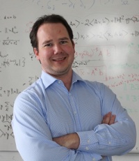
Holger Rauhut is Professor for Mathematics and Head of Chair C for Mathematics (Analysis) at RWTH Aachen University. Professor Rauhut came to RWTH Aachen in 2013 from a position as Professor for Mathematics at the Hausdorff Center for Mathematics, University of Bonn since 2008.

Professor Rauhut has, among many other things, written the book A Mathematical Introduction to Compressive Sensing together with Simon Foucart and published important research contributions about structured random matrices.

At the coming iTWIST workshop I am looking very much forward to hearing Holger Rauhut speak about low-rank tensor recovery. This is especially interesting because, while the compressed sensing (one-dimensional) or the matrix completion (two-dimensional) problems are relatively straightforward to solve, things start getting much more complicated when you try to generalise it from ordinary vectors or matrices to higher-order tensors. Algorithms for the general higher-dimensional case seem to be much more elusive and I am sure that Holger Rauhut can enlighten us on this topic (joint work with Reinhold Schneider and Zeljka Stojanac):

Low rank tensor recovery

An extension of compressive sensing predicts that matrices of low rank can be recovered from incomplete linear information via efficient algorithms, for instance nuclear norm minimization. Low rank representations become much more efficient one passing from matrices to tensors of higher order and it is of interest to extend algorithms and theory to the recovery of low rank tensors from incomplete information. Unfortunately, many problems related to matrix decompositions become computationally hard and/or hard to analyze when passing to higher order tensors. This talk presents two approaches to low rank tensor recovery together with (partial) results. The first one extends iterative hard thresholding algorithms to the tensor case and gives a partial recovery result based on a variant of the restricted isometry property. The second one considers relaxations of the tensor nuclear norm (which itself is NP-hard to compute) and corresponding semidefinite optimization problems. These relaxations are based on so-called theta bodies, a concept from convex algebraic geometry. For both approaches numerical experiments are promising but a number of open problems remain.

iTWIST’16 Keynote Speakers: Florent Krzakala

Note: You can still register for iTWIST’16 until Monday the 1st of August!

Our next speaker at iTWIST’16 is Florent Krzakala. Much like Phil Schniter – the previous speaker presented here – Florent Krzakala has made important and enlightening contributions to the Approximate Message Passing family of algorithms.

Florent Krzakala is Professor of Physics at École Normale Supérieure in Paris, France. Professor Krzakala came to ENS in 2013 from a position as Maître de conférence in ESPCI, Paris (Laboratoire de Physico-chimie Theorique) since 2004. Maître de conférence is a particular French academic designation that I am afraid I am going to have to ask my French colleagues to explain to me 😉

Where Phil Schniter seems to have approached the (G)AMP algorithms, that have become quite popular for compressed sensing, from an estimation-algorithms-in-digital-communications-background, Florent Krzakala has approached the topic from a statistical physics background which seems to have brought a lot of interesting new insight to the table. For example, together with Marc Mézard, Francois Sausset, Yifan Sun, and Lenka Zdeborová he has shown how AMP algorithms are able to perform impressively well compared to the classic l₁-minimization approach by using a special kind of so-called “seeded” measurement matrices in “Probabilistic reconstruction in compressed sensing: algorithms, phase diagrams, and threshold achieving matrices“.

At this year’s iTWIST workshop in a few weeks, Professor Krzakala is going to speak about matrix factorisation problems and the approximate message passing framework. Specifically, we are going to hear about:

Approximate Message Passing and Low Rank Matrix Factorization Problems

A large amount of interesting problem in machine learning and statistics can be expressed as a low rank structured matrix factorization problem, such as sparse PCA, planted clique, sub-matrix localization, clustering of mixtures of Gaussians or community detection in a graph.

I will discuss how recent ideas from statistical physics and information theory have led, on the one hand, to new mathematical insights in these problems, leading to a characterization of the optimal possible performances, and on the other to the development of new powerful algorithms, called approximate message passing, which turns out to be optimal for a large set of problems and parameters.

iTWIST’16 Keynote Speakers: Phil Schniter

With only one week left to register for iTWIST’16, I am going to walk you through the rest of our keynote speakers this week.

Our next speaker is Phil Schniter. Phil Schniter is Professsor in Electrical and Computer Engineering at Department of Electrical and Computer Engineering at Ohio State University, USA.

Professor Schniter joined the Department of Electrical and Computer Engineering at OSU after graduating with a PhD in Electrical Engineering from Cornell University in 2000. Phil Schniter also has industrial experience from Tektronix from 1993 to 1996 and has been a visiting professor at Eurecom (Sophia Antipolis, France) from October 2008 through February 2009, and at Supelec (Gif sur Yvette, France) from March 2009 through August 2009.

Professor Schniter has published an impressive selection of research papers; previously especially within digital communication. In recent years he has been very active in the research around generalised approximate message passing (GAMP). GAMP is an estimation framework that has become popular in compressed sensing / sparse estimation. The reasons for the success of this algorithm (family), as I see it, are that the algorithm estimates under-sampled sparse vectors with comparable accuracy to the classic l₁-minimisation approach in compressed sensing and favourable computational complexity. At the same time, the framework is easily adaptable to many kinds of different signal distributions and other types of structure than plain sparsity. If you are dealing with a signal that is not distributed according to the Laplace distribution that the l₁-minimisation approach implies, you can adapt GAMP to this other (known) distribution and achieve better reconstruction capabilities than the l₁-minimisation. Even if you don’t know the distribution, GAMP can also be modified to estimate it automatically and quite efficiently. This and many other details are among Professor Schniter’s contributions to the research on GAMP.

At this year’s iTWIST, Phil Schniter will be describing recent work on robust variants of GAMP. In details, the abstract reads (and this is joint work with Alyson Fletcher and Sundeep Rangan):

Robust approximate message passing

Approximate message passing (AMP) has recently become popular for inference in linear and generalized linear models. AMP can be viewed as an approximation of loopy belief propagation that requires only two matrix multiplies and a (typically simple) denoising step per iteration, and relatively few iterations, making it computationally efficient. When the measurement matrix “A” is large and well modeled as i.i.d. sub-Gaussian, AMP’s behavior is closely predicted by a state evolution. Furthermore, when this state evolution has unique fixed points, the AMP estimates are Bayes optimal. For general measurement matrices, however, AMP may produce highly suboptimal estimates or not even converge. Thus, there has been great interest in making AMP robust to the choice of measurement matrix.

In this talk, we describe some recent progress on robust AMP. In particular, we describe a method based on an approximation of non-loopy expectation propagation that, like AMP, requires only two matrix multiplies and a simple denoising step per iteration. But unlike AMP, it leverages knowledge of the measurement matrix SVD to yield excellent performance over a larger class of measurement matrices. In particular, when the Gramian A’A is large and unitarily invariant, its behavior is closely predicted by a state evolution whose fixed points match the replica prediction. Moreover, convergence has been proven in certain cases, with empirical results showing robust convergence even with severely ill-conditioned matrices. Like AMP, this robust AMP can be successfully used with non-scalar denoisers to accomplish sophisticated inference tasks, such as simultaneously learning and exploiting i.i.d. signal priors, or leveraging black-box denoisers such as BM3D. We look forward to describing these preliminary results, as well as ongoing research, on robust AMP.